From the Not Just Numbers blog:

Before we get into today’s post, a quick reminder that Mynda Treacy’s Excel Dashboards Course is closing on Thursday (8th May), so if you haven’t enrolled yet, you’ll need to be quick.

A couple of weeks ago, I posted a poll on the blog to see what versions of Excel we are all using. The poll is now closed, and the results make interesting reading.

First of all, the results themselves…

The question asked was, “Which version of Excel do you mostly use?”

This is not a proper statistical survey, just something to give a bit of an insight into what visitors to the blog are currently using.

Only 18% of us are sporting the latest model, ensuring that we can take advantage of the most up-to-date features.

Almost half (49%) are mostly using Excel 2010. This includes myself as I find it provides me with the right balance of up-to-date features and compatibility with what others are using (particularly important when you are building spreadsheets for others). The poll suggests to me that it is still probably the right version for me to use when developing for others.

Excel 2007 is about as popular as Excel 2013, and given it’s similarity to Excel 2010, I would expect it to have scored reasonably highly as there weren’t too many reasons to make the move from 2007 to 2010 – if you’d already made the move from 2003 to 2007.

11% are still using Excel 2003 or earlier, which Microsoft have now ceased to support. There has been a lot of reluctance among users to upgrade from this version as it was very stable and did everything most users would want. The most visible change in the next version was to introduce the ribbon menus, which didn’t add additional functionality but meant  a significant amount of training and/or experimentation was required to get up-to-speed on 2007 or later. I used as my main platform for development until quite recently.

As I mentioned in my earlier article, I think the withdrawal of Microsoft’s support might be the justification to bite the bullet and upgrade. I know a number of users who have jumped from 2003 to 2013. The learning curve isn’t really any greater than it would have been from 2003 to 2007.

Finally, as I suspected, very few of my readers are Mac users. I don’t use a Mac myself, so don’t really feel qualified to add much in the way of Mac related content. Obviously, much of the general Excel content applies and those who do use the Mac versions are very welcome on the blog. I know some of you do point out in comments when the Mac version does something different, which is much appreciated.

If you enjoyed this post, go to the top of the blog, where you can subscribe for regular updates and get two freebies “The 5 Excel features that you NEED to know” and “30 Chants for Better Charts”.

From the Not Just Numbers blog:

A reminder of a couple of looming deadlines before I get into today’s post:

Firstly, tomorrow is the last day to complete the poll on which version of Excel you use. Please complete the poll (at the top right of the blog) so that I can understand what readers are using.

Secondly, Thursday (May 1st) is your last chance to get Mynda Treacy’s Excel Dashboards course with a 20% discount. So, take a look now if you don’t want to miss out.

OK, on with today’s tip…

There are two ways you might want to capture and use the current date and/or time:

• Referring to the current date and/or time in a formula;
• Entering the current date or time in a cell

Ctrl+;   this enters the current date in the active cell

If you enjoyed this post, go to the top of the blog, where you can subscribe for regular updates and get two freebies “The 5 Excel features that you NEED to know” and “30 Chants for Better Charts”.

From the Not Just Numbers blog:

I hope everyone’s enjoyed the Easter Break.

Just a quick and easy tip this week to ease us all back in gently!

I’ve written a number of posts in the past about tidying up text using functions, e.g. (Simple tips for tidying up text in Excel and Removing all spaces from text), but I thought I’d give a quick mention to a useful tool for a one-off tidy-up that can be very powerful (and also works within formulae).

The Find and Replace tool appears throughout Microsoft Office, but within Excel it can be even more powerful.

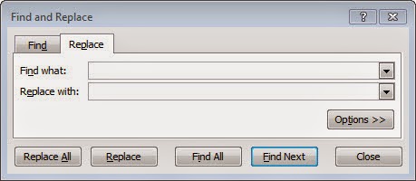
If you click the binoculars on the Home ribbon and choose Replace, you are presented with the following Dialog box:

• It will include text within the cells (it does not need to be the whole cell contents)
• It will look within formulae too
• It is not case sensitive (however the replacement text will use the case you have entered)

If you enjoyed this post, go to the top of the blog, where you can subscribe for regular updates and get two freebies “The 5 Excel features that you NEED to know” and “30 Chants for Better Charts”.

From the Not Just Numbers blog:

Last week, on the 8th April 2014, Microsoft withdrew support for Office 2003 and Windows XP, including, of particular interest to readers of this blog, Excel 2003.

The effect of this depends on two factors:

• How many people/organisations are still using Excel 2003?
• What are the implications for those that are?

If you enjoyed this post, go to the top of the blog, where you can subscribe for regular updates and get two freebies “The 5 Excel features that you NEED to know” and “30 Chants for Better Charts”.

From the Not Just Numbers blog:

Just a very short tip for this week.

Do you ever have a situation where you need to compare two values but you don’t want to treat them as the same if one is upper case and the other is lower case?

As far as Excel is concerned, “A”=”a”!

Fortunately, there is a function in Excel that can help.

The EXACT function allows you to compare two values and returns TRUE if they are EXACTLY the same, including case.

So,

where

=IF(“A”=”a”,”The same”,”Different”)

returns “The same”

=IF(EXACT(“A”,”a”),”The same”,”Different”)

returns “Different”

That’s it! Simple, but handy if you need it.

If you enjoyed this post, go to the top of the blog, where you can subscribe for regular updates and get two freebies “The 5 Excel features that you NEED to know” and “30 Chants for Better Charts”.

From the Not Just Numbers blog:

One of the biggest challenges when dealing with lists of data is spotting and/or removing duplicate entries.

Fortunately, the more recent versions of Excel offer some excellent tools for handling this problem.

I thought that this week, I would give you a quick introduction to them.

Highlighting Duplicates

Excel offers a quick facility to highlight duplicate entries in a list.

Simply highlight the list and, from the Home ribbon, select Conditional Formatting, Highlight Cells Rules, Duplicate Values.

You then get two drop-down boxes to choose whether you want to highlight the duplicates or the unique values and what colours you want to highlight them in. It’s as simple as that.

This will simply highlight all of the cells that have a duplicate (or don’t, if you select unique values).

Removing Duplicates

Often, you don’t need to see the duplicates, just get rid of them. Excel also has a tool for that, which is also a little more sophisticated than the previous tool.

It doesn’t just look at duplicate cells, but duplicate rows.

To use the tool, highlight all of the columns containing your data (data should be formatted correctly as covered in my earlier post on this subject, or at least with a column for each field and a row for each record).

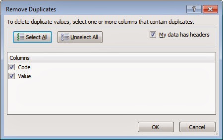
On the Data ribbon, select Remove Duplicates and you will see the following dialog box:

If you enjoyed this post, go to the top of the blog, where you can subscribe for regular updates and get two freebies “The 5 Excel features that you NEED to know” and “30 Chants for Better Charts”.

From the Not Just Numbers blog:

No matter how much we think we know Excel, we still come across new things all of the time.

This is one a client showed me the other day – and it’s a neat little trick!

How many times have you had a column of codes that Excel is reading as numbers and you need to be read as text (to work with a VLOOKUP or SUMIF for example)?

You can change the number format to text but this only partly solves the problem. It means any future numbers entered will be seen as text, but Excel only reads the existing codes as text once you have hit F2 and return on each one. I’ve found myself rattling down many a column like this in the past.

This little tip, however, means that I never have to do that again!

The approach involves using the Text to Columns feature that is designed for breaking text out into columns. The final step of the wizard, however, allows you to specify the format of each resulting column. This is how this tip works.

Simply follow the following steps:

• Highlight the column of numbers;
• Click Data, Text-to-Columns;
• Select Delimited and click Next;
• And Next again;
• Select Text as the column data format;
• Click Finish.

If you enjoyed this post, go to the top of the blog, where you can subscribe for regular updates and get two freebies “The 5 Excel features that you NEED to know” and “30 Chants for Better Charts”.

From the Not Just Numbers blog:

I’ve just got another short post for you this week, that’s a follow-up to a post I wrote a few years’ back.

Back in 2009, I wrote a post about Excel’s Solver Add-In, which enables you to essentially reverse engineer an excel spreadsheet.

It allows you to take an existing spreadsheet, set a target for the result of the spreadsheet, and identify what inputs will achieve that target while satisfying any constraints you specify.

For more details on what the Solver Add-In does, take a look at the earlier post.

While working on a client’s spreadsheet last week, I came across one of the Solver Add-In’s biggest limitations – and here’s how I got around it…

I was working on a spreadsheet to pick the optimum Fantasy Football team, and realised that I could have anything up to 500 players to choose from – meaning that there were 500 variables in the Solver model. It was at this point that I discovered that the Solver Add-In restricts the number of variables to 200!

Fortunately, after a little Googling, I found this:

OpenSolver for Excel
The Open Source Optimization Solver for Excel

This is a free Add-In for Excel, developed and maintained by Andrew Mason and students at the Engineering Science department, University of Auckland, New Zealand.

It works very similarly to the standard Solver Add-In, however, crucially, it does not have this artificial limit of 200 variables.

If you’ve never used the Solver Add-In, I would recommend that you take a look. If you have, but have a problem that requires over 200 variables, you could do worse than downloading OpenSolver.

Have fun!

If you enjoyed this post, go to the top of the blog, where you can subscribe for regular updates and get two freebies “The 5 Excel features that you NEED to know” and “30 Chants for Better Charts”.

From the Not Just Numbers blog:

Just a short post this week, as I have a pretty manic workload at the moment!

A few years ago, I did a post on using Data Validation to produce drop-down lists. However, Data Validation allows for many other ways to control the data entered and I thought I would cover one of those here – how to control the entry of dates to within a certain range.

To open the Data Validation window, select the range that you want to apply the validation to and click Data Validation on the Data ribbon (select Data Validation from the resulting drop-down).

From the “Allow” drop-down at the top of the window, select Date, choose what the operator from the next drop-down (there a number of options here such as greater than, less than, etc. but in most cases we will choose “between”).

We then enter the earliest and latest dates that we wish to allow. e.g.

It would be good practice to enter these as cell references and to enter the dates in the cells, so that the range is clearly visible and can be edited by a user.

This will present the user with an error message if they try to enter a date outside of this range (or if they try to enter anything that isn’t a valid date at all), and will not allow them to leave the cell without entering a valid date within the range.

As with all Data Validation, you can use the other two tabs to enter an Input Message that will appear when you click in the cell and/or create a custom Error Alert for when the data entered is invalid.

If you enjoyed this post, go to the top of the blog, where you can subscribe for regular updates and get two freebies “The 5 Excel features that you NEED to know” and “30 Chants for Better Charts”.

From the Not Just Numbers blog:

Excel’s conditional formatting feature typically allows you to set the format of a cell based upon its contents, and allows you to define all sorts of rules upon which to do this.

This is great, but what if you want the cell’s format to be based upon the contents of a different cell (or cells)?

A typical use for this might be for a traffic light graphic giving a quick visual aid to understanding a set of numbers.

Fortunately Excel provides a relatively straight-forward way of doing this.

The answer is to use the formula option in Conditional Formatting.

Highlight the cell, or range of cells, that the conditional formatting is to be applied to.

Select Conditional Formatting from the Home ribbon and select “New rule”. Then select the bottom option from the list – “Use a formula to determine which cells to format”:

You can then type a formula into the box that will be used as the criteria to determine whether each cell is to be formatted, or not.

The criteria should start with an “=” sign and then follow the same rules as the condition argument of an IF function.

Where you are applying the conditional formatting to more than one cell, the criteria should be written from the perspective of the top left cell of the range being formatted. This becomes important in how it will treat relative cell references. Cell references can be made absolute using the dollar sign, as in a regular Excel function.

Once you are happy with your criteria, click the Format button and set the formatting that you want to apply should the criteria be met.

Some examples should make this a little clearer…

Let us take a simple one first. Say we wished to fill cell C3 with a red background, if cell A1 was negative.

We would click in cell C3 and open the dialog box as above. We then enter the following into the criteria box:

=A1<0

We then click the format button and select a red fill.

As we are only formatting one cell, it doesn’t matter whether we use dollar signs or not.

Now, let’s say we want the whole range C1:G10 to be coloured red if A1 is negative.

We would select the range C1:G10, and then do the same as before, however now we need to consider how we want cells other than the top left cell of the range to be treated.

In this case we want them to still look at the contents of A1 so we will need to fix the reference to A1 by adding the $ sign in front of both the row and column reference. Our criteria should therefore read:

=$A$1<0

If we didn’t add the $ signs, then the criteria would be looking at a different cell each time.

C1 would be looking at A1 (as C1 is the top left cell in the range), however C2 would be looking at A2, D1 would be looking at B1 and D2 would be looking at B2, etc.

We may want the reference to be relative in other cases. Say we wanted to apply the conditional formatting to the same range, C1:G10, but this time wanted to fill the row (columns C to G) red when the contents of column A is negative.

We would do exactly as above but this time apply the dollars as follows:

=$A1<0

We are still fixing the column but not the row, so now C1 will look at A1 (as before), and D1, E1, F1 and G1 will also look at A1 as we have fixed the column to always be A. However C2 to G2 will all look at A2 as the row reference is still relative.

The criteria you use can refer to more than one or a range of cells, so it could be any of the following:

=SUM(A1:A10)>=10,000
=A1-B1=0
=A1>B1
=SUM(A1:A10)>B1

Basically anything you could have entered as the criteria in an IF function (with an “=” sign in front of it).

You can also apply more than one rule to the same cell, so to apply our traffic light system, for example, we might have the following rules:

• The ordinary format of the cell set to an amber (or orange fill) so that the fill is this colour if the other rules don’t apply. You don’t need Conditional Formatting for this;
• New Rule =A1>=500  to give a fill of green
• New Rule =A1<=-500 to give a fill of red

If you enjoyed this post, go to the top of the blog, where you can subscribe for regular updates and get two freebies “The 5 Excel features that you NEED to know” and “30 Chants for Better Charts”.