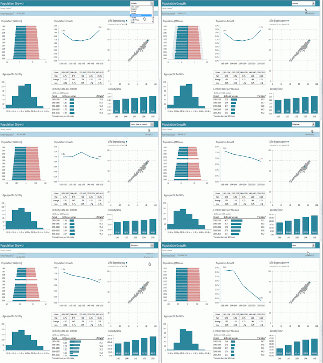
Monthly close always overruns? Just like 90% of finance staff

Month EndFrom the Not Just Numbers blog:

As a response to last week’s post on the automation of management accounts, I was approached by Adra Match, Data Matching and Reconciliation Software experts with an offer of a blog post about their research on the month-end process, which makes for some interesting reading.

Whether it is automation of the accounts preparation process (as per last week’s post) or automation of reconciliations (as provided by Adra Match’s software), from these results, it would appear that we need all of the help we can get!

Here’s the post…

Monthly close always overruns? Just like 90% of finance staff

A guest post by Alan Bagnall of Adra Match

There is always a compromise between speed and accuracy, rarely can they co-exist. More speed means less quality – and the month end close is the epitome of this.

Pressure seems to be on for finance staff to complete the month end close process faster, according to a new Adra Match survey of European and US financial accounting professionals. The monthly close process was voiced as “a mad dash’ by a number of the finance professionals surveyed, a sentiment most, if not all financial accounting professionals can relate to.

That “mad dash’ also means that in over 70% of cases financial reports aren’t being filed for at least four days past the deadline. If manually processed accounts are open longer than they should be, your business might be in for trouble: The business becomes exposed to risk, it will certainly run into problems with your local regulator, and it has the risk of having material misstatements which is a heftier challenge today than before. It’s now illegal to rely on your auditor to spot errors!

One finance processional who took part in the survey voiced the significant pressure faced by finance staff :

“my objective is to achieve a faster, more reliable close, make it efficient”.

>>>Download the free financial close report infographic for an overview of the survey results  <<<

As well as a speedier turnaround of month end figures, participants also listed the following as being among the top priorities for the finance department:

  • Increased reliability
  • Reduced risk
  • Segregation of duties
  • And a transparent audit trail

Of those points, reliability of the close process appears to be the main challenge for most US and European financial accounting professionals: A mere 28% of finance staff trust the reported numbers.

So most financial staff working directly with the raw data don’t trust their own reported numbers. These are horrible facts. Horrible, because the numbers reported in our balance sheet and profit & loss statements, are believed to be correct. While this survey proves exactly the opposite.

The report also reveals that one other key area for concern is risk in the account reconciliation process. One reason for this may be that a vast amount of finance staff with too many reconciliations to perform only use spreadsheets to reconcile their accounts. While spreadsheets when used correctly can work with you, often they do not track which user has made which changes, making the separation of duties difficult, if not impossible, to monitor.

Doesn’t it seem strange that while finance departments use technology to automate a lot of their processes, the use of technology in the account reconciliation process has hardly progressed since the 1980s? Why?

  • Isn’t it time to bring the arduous account reconciliation challenge into the digital age too? With an automated “Balance Sheet Reconciliation Process” solution?

Don’t forget, if you want to read the full survey results you can at the link below:

Adra Match financial benchmark survey results.

Excel Expert Course

If you enjoyed this post, go to the top of the blog, where you can subscribe for regular updates and get two freebies “The 5 Excel features that you NEED to know” and “30 Chants for Better Charts”.


Excel Tip: Are you responsible for producing Management Accounts or Monthly Reports?

Head Against WallFrom the Not Just Numbers blog:

I know that many of you, like me, are accountants and a large number of you, no doubt, are responsible for producing monthly management accounts. I’m sure that many of you that aren’t accountants, as Excel users, are responsible for producing some kind of regular monthly, weekly or daily report.

This week’s post is more of a plea, to take a moment out of your busy schedule to stop and have a think about how you go about this regular reporting.

How long do you spend on this each month/week/day?

How long do you think you should be spending?

Let me give you some food for thought.

Is the data for your reports in the same place each month?

Are the reports you’re required to produce in the same format every month/week/day?

It is very rare that the answer to either of these questions is no. For example, if we are talking about management accounts, the data is held in the accounting system in exactly the same format as it was last month – and the management accounts are produced in the same format as last month, usually in an Excel template.

Given Excel’s ability to manipulate data – and perform the same manipulations time and time again, why would the process of producing these reports take more than a few seconds?

Simply create an Excel template that converts the raw data into the final report, and just paste or import the new raw data in each month!

Whichever way you go about it, I urge you to stop and think. Logically, it should only take a few seconds. Any longer means that you are manually doing things every month/week/day that Excel could be doing for you.

If you need any help, I have covered this in more detail previously.

My very first post on this blog (back in September 2008!) was on this subject and gives a brief overview of how you can go about this for a set of management accounts:

Do your management accounts take weeks, days, hours, minutes…or seconds to prepare?

and more recently (November 2013) I wrote a far more detailed explanation of the process in a publication published by the IT Faculty of the Institute of Chartered Accountants in England & Wales (ICAEW) entitled:

Automating management accounts production in Excel: a simple approach

(This is free to members of the IT Faculty or the ICAEW’s Excel community or £25 to purchase for everyone else, from the ICAEW at the link above).

If you want, I can even set it up for you as this is a job that I have done for many clients over the years.

Whatever you do, I urge you not to just go back to a time-taking and unnecessary monthly/weekly/daily process.

Excel Expert Course

If you enjoyed this post, go to the top of the blog, where you can subscribe for regular updates and get two freebies “The 5 Excel features that you NEED to know” and “30 Chants for Better Charts”.

Excel Tip: Editing multiple formulae

Change EverythingFrom the Not Just Numbers blog:

I’ve got a simple tip this week that you have probably used elsewhere, but most Excel users I meet do not know that it can be used for this purpose.

This is a nice little trick for that situation when you need to make the same change to many formulae in different cells.

This can be a very time-consuming task, particularly if the spreadsheet has not been well-structured in the first place. If it has, at least all variables, etc. should have been referenced to cells rather than hard-coded in the formula. See my earlier post for some principles on good spreadsheet practice.

Sometimes though, you’re stuck with making a change like this. The good news is that a simple tool that is available throughout Microsoft Office can be used.

This tool is the Replace facility.

Many of you will have used this to replace text in a Word document, or maybe you’ve used it in an Excel document, but did you know that it works exactly the same within formulae?

Yes, say you have a range of formulae that refer to cell A1 for a particular variable and you need them to now refer to cell B3. You can use Replace to make the change.

Simply highlight the range with the formulae that need changing, click the binoculars on the Home ribbon and choose Replace and fill the boxes in as below:

Click Replace All and Excel will replace the text A1 with B3 throughout all of the formulae.

Note of caution:

This is a simple text replace, so is not intelligent. For example:

$A$1 will not be changed
A113 will become B313

Having said that, with a little thought about the consequences beforehand, you can usually do the Replace in such a way that will solve your problem.

Excel Expert Course

If you enjoyed this post, go to the top of the blog, where you can subscribe for regular updates and get two freebies “The 5 Excel features that you NEED to know” and “30 Chants for Better Charts”.

Excel Tip: Using the HYPERLINK function

HYPERLINKFrom the Not Just Numbers blog:

Two events of note occurred over the weekend:

1. My local football team (Sunderland AFC) beat our bitter rivals (Newcastle United) 3-0 at their place for the second year in a row!

2. I responded to a blog comment asking how to make a URL in Excel that was the result of an IF statement a clickable hyperlink.

I will endeavour to make this post about the latter, but please forgive me if I find it difficult to avoid mentioning the former!

The HYPERLINK formula in Excel allows returns a clickable hyperlink as its result. It is used as follows:

=HYPERLINK(Link,[Friendly name])

Link can be a URL, a file path, or a reference to a cell or range in this or Excel or Office document and should be included in quotes (unless it’s a reference to the text rather than the text itself).

[Friendly name] is an optional argument, that allows you to choose what text appears in the cell. If you don’t enter this argument, the link text shows. Again, this should be in quotes (unless it’s a reference to the text rather than the text itself).

Some examples:

=HYPERLINK(“http://www.safc.com”,”Sunderland AFC”) displays the text Sunderland AFC in the cell and links to the team website when you click on it.

=HYPERLINK(“C:\Budgets\2014 Budget.xlsx”,”Open budget spreadsheet”) displays the text Open budget spreadsheet and opens the 2014 Budget spreadsheet from the Budgets folder on the C drive when you click on it.

=HYPERLINK(“[2014 Budget.xlsx]Assumptions!E46″,”Edit inflation”) displays the text Edit inflation and goes to cell E46 on the Assumptions worskheet of 2014 Budget.xlsx. This format should be used for linking even within the same spreadsheet.

This function really comes into its own though when you populate these arguments with references to results as the links can then be dynamically generated from the contents of the spreadsheet.

For example:

=HYPERLINK(B5,A5) will display whatever text is held in cell A5 and link to the URL or path contained in cell B5

Or potentially more usefully:

=HYPERLINK(“http://www.bbc.co.uk/sport/football/teams/”&A5,A5) which will display the football team name held in cell A5 and link to that team’s news page on the BBC website. e.g. if A5 contains the text sunderland, the link will go to http://www.bbc.co.uk/sport/football/teams/sunderland whereas if A5 contains newcastle-united it will go to http://www.bbc.co.uk/sport/football/teams/newastle-united.

See my earlier post about manipulating text in Excel to explain use of the Ampersand (&) character.

You could also use VLOOKUPIF statements or any other functions to populate the arguments of the HYPERLINK function and create dynamic links.

There, I hardly mentioned the score!

Excel Expert Course

If you enjoyed this post, go to the top of the blog, where you can subscribe for regular updates and get two freebies “The 5 Excel features that you NEED to know” and “30 Chants for Better Charts”.

Excel Tip: Remove old items from PivotTable drop-down lists

Clean listsFrom the Not Just Numbers blog:

Just a short post this week on something I only discovered myself the other day.

Before we get into the post though, just a quick reminder that Mynda Treacy’s Dashboards Course will be closing on Thursday, so if you haven’t already purchased it and don’t want to miss out, get yourself over there now, before it’s too late – you will also receive a free copy of my Introduction to PivotTables course. You won’t regret it.

This week’s post was prompted by a question from a client who was baffled by items appearing in the drop-down selection boxes in his PivotTables that were no longer in the data being referenced.

This was a particular problem as the PivotTables were being sent out to individual salespeople reporting on their own data – but because the pivot tables had previously been looking at the whole data set, all of the other salespeople’s customers were appearing in the drop-down lists.

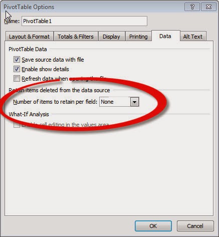
I wasn’t quite sure myself why this was happening at first, but going through the PivotTable options (accessed by right-clicking on the PivotTable and selecting PivotTable Options…), I discovered the following setting on the Data tab:

Retain items deleted from the data source…Number of items to retain per field

This setting is by default set to Automatic and changing it to None will stop the PivotTable retaining these items in the drop-down lists (they will disappear the next time you click Refresh). It’s as simple as that – once you know that the setting is there!

Post Script

Out of curiosity, I tried to find out what the three possible settings are supposed to do (the third setting is Max). Microsoft Excel help was not particularly enlightening on the subject:

Retain items deleted from the data source section
Number of items to return per field    To specify the number of items for each field to temporarily cache with the workbook, select one of the following:

Automatic     The default number of unique items for each field.
None     No unique items for each field.
Max     The maximum number of unique items for each field. You can specify up to 1,048,576 items.

It does not give any indication what the default number is or how you specify the maximum!

A search around the web didn’t bring up any further clarification, but I’m sure some of our clever readers can elaborate, so please add a comment if you know what the difference is between the Automatic and Max settings!

Excel Expert Course

If you enjoyed this post, go to the top of the blog, where you can subscribe for regular updates and get two freebies “The 5 Excel features that you NEED to know” and “30 Chants for Better Charts”.

Guest Post – Calculating Median and Mode in Excel


This week you’ve got a break from me with a very useful guest post from Alan Murray of Computergaga.

Before we get into that though, just a quick reminder that the early bird discount on Mynda Treacy’s excellent Excel Dashboards course expires on Thursday, so if you don’t want to miss out, click over there now.

OK, on with Alan’s tips for when you don’t just want the average AVERAGE!

Calculating Median and Mode in Excel

When calculating averages in Excel, this normally involves using the AVERAGE function. The AVERAGE function in Excel calculates the mean of a set of numbers.
There are two other types of averages known as median and mode. Let’s take a look at calculating median and mode in Excel.

Calculating the Median

The median is the middle number in a sorted list of numbers. If you were to calculate the median with a pen and paper you would have to;

  1. Write down the list of numbers in numerical order.
  2. If there were an odd number of results, then the median would be the middle number.
  3. If there were an even number of results, then the median would be the mean of the two central numbers.
Fortunately Excel can handle all of this for us with the MEDIAN function. The following formula can be written to calculate the median from the list of exam scores.
=MEDIAN(B4:B13)

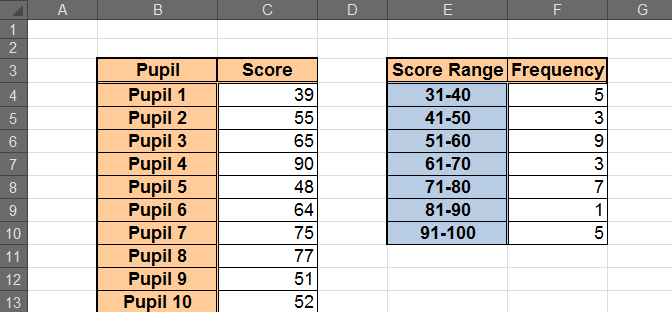
The list of exam scores is not sorted in numerical order, but that is no problem for Excel. The median has been found by finding the mean of 55 and 65 because there are 10 scores which is an even number of results.
39, 48, 51, 52, 5565, 75, 77, 77,90
(55 + 65) / 2 = 60

Finding the Mode

The mode, or modal number, is the number that occurs most frequently in a list. There can be more than one mode.
In Excel, the MODE function can be used on a list to return the number that occurs most often. In this example the formula would look like below.
=MODE(B4:B13)
The mode in this example can easily be seen to be 77 as it is the only one to appear more than once. If there is more than one modal number, this formula will only return the first one.

Returning Multiple Modes

To return multiple modes the MODE.MULT function can be used. This function was released with Excel 2010 so is not available on versions previous to that.
This function is an array function, so to run the function you should press Ctrl + Shift + Enter instead of only Enter. It will also appear in the Formula Bar wrapped within curly braces.
You will need to select a range of cells to apply the function to, or copy the formula and run it again.
In the example below there are 3 modal values. The following MODE.MULT function has been used in cells D5:D7 to return the results.

{=MODE.MULT(B4:B18)}


When there are no more modal values the function will return the #N/A error.

Watch the Video


Create a Frequency Distribution Table

Results are often broken down into groups, or classes. This
frequency distribution table gives us a good view of the spread of our data and
also identifies the class with the most occurrences, known as the modal class.
The table below shows the grades of 34 pupils in range
C4:C37. 


The COUNTIFS function has been used to calculate these
frequencies. The formula below was entered into cell F4 and then copied to the
other cells of the table, with the criteria altered to match the class. 


The formula counts the number of scores that are greater
than or equals to 31, but less than 40. This is then repeated for each class.
The COUNTIFS function was released with Excel 2007. If you
are using a version previous to this, the SUMPRODUCT
function could be used to count based on multiple conditions.
.


About the author:
Alan Murray is an IT Trainer and the founder of Computergaga. Author of the
popular Computergaga Blog providing the latest Excel, Word, PowerPoint and Project tips and techniques.
Excel Expert Course
If you enjoyed this post, go to the top of the blog, where you can subscribe for regular updates and get two freebies “The 5 Excel features that you NEED to know” and “30 Chants for Better Charts”.

Excel Dashboards Online Course – Limited time offer

Excel DashboardsFrom the Not Just Numbers blog:

A number of you will remember that I have previously recommended Mynda Treacy’s Excel Dashboard course(many of you purchased it), and I’m pleased to tell you that it is once again available – for a limited time.

The course is video based and available online 24/7. It comes with comprehensive Excel workbooks and several sample dashboards to keep. There’s also an option to download the videos, plus Mynda personally provides support for the first 6 weeks of the 12 month membership.

Dashboards are an incredibly valuable tool in today’s market for consultants, analysts, managers and accountants. But Excel doesn’t make it straightforward to build highly professional and interactive dashboards. That’s why this type of training is crucial.

What readers are saying about the course:
The previous classes have been a huge hit with many people saying how they love the cool
techniques and how they’ve been able to impress their colleagues and clients by using them in all
sorts of reports, not just dashboards.

Others have said the course has prompted them to take a whole new approach to producing their monthly reports.

I highly recommend the course but don’t take my word for it. You can read comments from past students and find out more (including sample videos) here.

Bonus 20% Off (and a free gift)
If you join the class by January 23rd you can get it for 20% off plus I’ll include my Introduction to Pivot Tables video training course absolutely free, just enter FEECHAN in the ‘Referral Source’ field below the PayPal Buy Now button when you purchase Mynda’s course and then email me your receipt.

So, do yourself a favour and check out the course. The price is incredibly fair, the course is excellent and it’ll transform your Excel reports and possibly even your Excel career.

Learn Excel Dashboard Course

Disclosure: I make a small commission for students who join Mynda’s course, but as you know I
don’t just recommend anything and everything. It has to be of outstanding quality and value, and
something I can genuinely recommend. After all, if doesn’t live up to what I’ve promised you’ll think poorly of me too and I don’t want that. Oh, and just watching the course videos won’t transform
your career, you have to actually put it into practice, but then you know that.

Excel Expert Course

If you enjoyed this post, go to the top of the blog, where you can subscribe for regular updates and get two freebies “The 5 Excel features that you NEED to know” and “30 Chants for Better Charts”.

Excel Tip: The structure of every Excel function

2014From the Not Just Numbers blog:

As this is my first post of 2014, I must start by wishing all of my readers a very Happy New Year, and thank you all for making 2013 the most successful yet for Not Just Numbers.

I have explained hundreds of Excel functions on this blog, and, in one post, covered how to access every function in Excel, but it occurred to me that I have never covered the universal way that every Excel function works, so I thought that would be a useful way to start the New Year.

Every function in Excel follows exactly the same format, and when you understand that, it makes it much easier to pick up new functions.

The basic format of an Excel function is the name of the function, followed by its arguments in brackets and separated by commas:

=FUNCTIONNAME(argument1,argument2…)

I have included the equals sign (=) in front of the format above but this is not strictly part of the individual function. The equals sign (as the first character in a cell) tells Excel that the contents of that cell are to be evaluated. So, if the function was entered in a cell on its own, it would need the equals sign – however if the function was used within another function or calculation, you would not repeat the equals sign.

The arguments of the function are the values that it needs to know in order to calculate. The number of arguments will differ depending on the function. Some functions also have optional arguments (in the Excel help files, these are shown in square brackets.

Let’s take the IF function as an example. In programming, an IF statement would normally follow the following syntax:

IF logical_test THEN value_if_true ELSE value_if_false

However, in Excel, it must follow the Excel format for all functions as described above, so the three arguments are separated by commas in brackets after the function name, i.e.

IF(logical_test,value_if_true,value_if_false)

Its format, according to the Excel help files, is:

IF(logical_test, [value_if_true], [value_if_false])

As we can see, only the first argument is required (logical_test) the other two being optional (value_if_true and value_if_false).

What is acceptable for each argument will depend on the function in question, but in this case, logical_test is an expression that can be evaluated as true or false, whereas value_if_true and value_if_false can be any value (numbers or text) or any calculation resulting in a value.

So some acceptable IF statements could be:

=IF(A1=10) returns TRUE if A1=10, or FALSE otherwise

=IF(A1=10,”Yes”,”No”) returns Yes if A1=10, or No otherwise

or even,

=IF(A1=10,”Yes”,IF(B1=5,”Yes”,”No”)) returns Yes if A1=10, but if A1 doesn’t equal 10,  it returns Yes if B1 is 5 but No otherwise.

Yes, functions can be used as arguments for other functions (including other instances of the same function – as in this example).

The last example is a Nested IF statement. Don’t worry if you haven’t followed fully how the IF statement works, as this was not the point of this post. You can read more about the IF statement here.

The important thing is that you understand the structure of Excel functions in general.

Excel Expert Course

If you enjoyed this post, go to the top of the blog, where you can subscribe for regular updates and get two freebies “The 5 Excel features that you NEED to know” and “30 Chants for Better Charts”.
Excel Tip: Quickly reverse the sign of a block of numbers

PostiveNegativeFrom the Not Just Numbers blog:

This week’s tip is a nice simple one that I only discovered a few weeks back when a client needed to reverse the sign on a large block of entered data.

For those of you that might not get to the tip this week (believe it or not, Excel is not always at the top of everyone’s priority list over the Christmas break!), I hope you have all had a great Christmas, and I wish you all a Happy and Productive 2014!

If you want to make 2014 even more productive, why not treat yourself to a year of Excel Email support for just £75 (or $112.50 if you prefer).

Festivities and shameless plug over! On with today’s tip…

The client in question had a range of numbers in Excel entered as positive figures that to be consistent with other reports should have been negatives (it was the expenses section of a budget spreadsheet and all other group companies had set their budgets up with costs entered as negatives).

I was going to enter a formula in a blank area of the spreadsheet (e.g. =-A1, where the range to be reversed starts in cell A1) and copy this over a range the same size as the range in question. I could then copy this and paste as values over the original range. I then stopped myself and wondered if it could be done in one step. A quick look around in the Paste Special dialogue box confirmed it could.

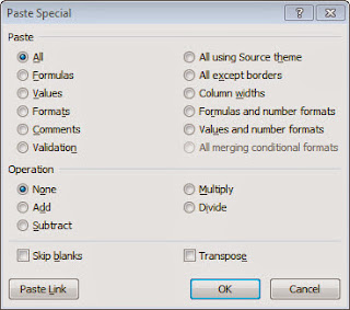
When you select Paste, Paste Special you are presented with the following dialogue box:

It is the section entitled “Operation” that caught my eye. This takes the pasted number and applies the selected operation to that and the existing contents of the cell.

So all we need to do is:

  • enter -1 in a blank cell
  • copy this cell to the clipboard
  • highlight the range of cells that we want to reverse
  • click Paste Special
  • Select Multiply under Operation and click OK

Nice and simple. It also has the added advantage that it will leave any formulae intact in the destination range (this would not have been the case in my first approach).

OK, back to the celebrations, see you in 2014!

Excel Expert Course

If you enjoyed this post, go to the top of the blog, where you can subscribe for regular updates and get two freebies “The 5 Excel features that you NEED to know” and “30 Chants for Better Charts”.

Partridges, Pear Trees and Merry Christmas!

Christmas QuestionFrom the Not Just Numbers blog:

Last week’s post caused a bit of a stir – and distracted a lot of people from work in the run up to Christmas!

In case you missed it, here is the post:

A Christmas Excel Challenge

I asked readers to come up with ways of using Excel to calculate how many gifts are in the Christmas song, The Twelve Days of Christmas, and, boy, did you rise to the challenge!

You can read all of the comments on the post itself, but I have highlighted below some of my favourites.

Just for clarification, there was no trick, each days gift was considered as one gift, e.g. a Partridge in a Pear Tree is one gift (not one Partridge and one Pear Tree). However, each gift (apart from the last) is received on more than one day, the Partridge in a Pear Tree being received on each of the 12 days, the two Turtle Doves being received on the each of the last 11 days, etc.

For most people (myself included) the maths skills stopped at coming up with a formula for each day’s presents:

=(B1+1)/2*B1

where B1 contains the day number in question. Therefore on the 12th day 78 gifts are received.

However, Simon Thacker was the first to come up with one formula for the total number of gifts:

=B1*((B1+1)*(B1+2))/6

returning 364 total gifts over the 12 days.

This is a Tetrahedral number from Pascal’s Triangle, as described in this video from Mary Pat Campbell explaining the formula above.

No doubt that this is the most efficient solution, with just one formula to calculate the answer.

This was, however, an Excel problem rather than a maths problem, so I think it is also worth mentioning a more Excel-based solution from Ray Andrews:

“I just like the simplicity of numbering 1 to12 in row 1, 12 to1 in row 2, multiplying row 1 by row 2 in row 3 and summing the result of row three in the thirteenth column”

This uses Excel’s capabilities while keeping the maths really simple.

Finally I did say that I would mention quirky solutions too and my favourite is this from Mike McCormick:

=COUNTIF(range,”*Partridge*”)*1+COUNTIF(range,”*Turtle*”)*2+COUNTIF(range,”*French*”)*3+COUNTIF(range,”*Calling*”)*4+COUNTIF(range,”*Golden*”)*5+COUNTIF(range,”*Geese*”)*6+COUNTIF(range,”*Swans*”)*7+COUNTIF(range,”*Maids*”)*8+COUNTIF(range,”*Ladies*”)*9+COUNTIF(range,”*Lords*”)*10+COUNTIF(range,”*Pipers*”)*11+COUNTIF(range,”*Drummers*”)*12

Where range contains the lyrics. of the song!

Thanks for all of your contributions.

Have a wonderful Christmas and a fantastic New Year!

Glen

Excel Expert Course

If you enjoyed this post, go to the top of the blog, where you can subscribe for regular updates and get two freebies “The 5 Excel features that you NEED to know” and “30 Chants for Better Charts”.