Excel Tip: Don’t do this with your table headings!

From the Not Just Numbers blog:

Another quick tip this week. This time it is a little bugbear of mine that I often see done by people not realising the problems it can cause them later.

It is really simple to get right if you know you need to!

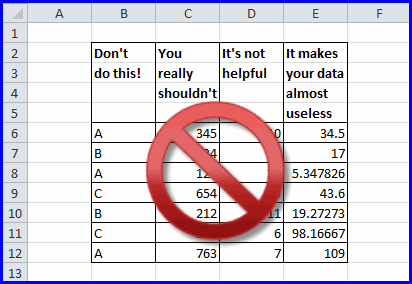
See if you can guess what it is from the image. If you can’t, I would recommend that you read on.

The problem is entering multi-row titles on any table of data.

I am not just talking about the table feature in Excel, but any table of data, such as the one in the picture.

In an earlier post I wrote about how to lay out data to make it useful.

The table format above fits all of these requirements, but falls down on the headings. Simply because you have used more than one line for the heading, it won’t work properly if you decide you want to use AutoFilter, or a PivotTable!

This is really simple to avoid.

You can type the heading on one row and then apply word wrap to the cells on that row (select “Wrap Text” from the Home ribbon). If you want specific line breaks in the text, you can use Alt+Enter to insert a line break within the cell.

The data then fits all of the criteria to be used in a PivotTable, or to enable AutoFilter.

That’s it – I’ll get off my soap box now!

Don’t forget that Mynda Treacy’s Excel dashboards course will be available again soon for a short period of time. If you’re not subscribed to the blog, do so now (at the top right of the blog) so that I can let you know when it’s available – and to be notified of future Excel Tips.

If you enjoyed this post, go to the top of the blog, where you can subscribe for regular updates and get your free report “The 5 Excel features that you NEED to know”.

From the Not Just Numbers blog:

Just a short post today because I have a very tight deadline to meet on a publication I am writing for the ICAEW (The Institute of Chartered Accountants here in England) on Automating Management Accounts in Excel.

Before we get into the post though, I have some exciting news for those of you who missed out on Mynda Treacy’s Excel Dashboards course last time around. The course will be made available again for a limited time later this month. In the meantime, you can (re)read Mynda’s guest post on the subject of Excel Dashboards here.

If you want to make sure you don’t miss out this time, ensure that you are subscribed to the blog as I will keep subscribers updated. If you are not a subscriber, you can do so by leaving your email address in the form at the top right of the blog.

Today’s post is a quick tip on how to use the current time and date in Excel.

There are two very similar functions that Excel provides for this – NOW and TODAY.

Both functions have no arguments but must still be followed by the (empty) brackets.

=NOW() returns the current date and time

=TODAY() returns the current date (actually it returns midnight at today’s date)

I covered how Excel handles dates and time in a post a couple of weeks ago. Looking at the functions in those terms – NOW returns the full serial number for the current date and time and TODAY returns that serial number rounded down to the nearest whole number,

This functions can be used on their own, or as values in formulae, e.g using =TODAY()-A1 to calculate the elapsed time since the date in A1.

One caution to add to using these functions is that the values only update when Excel recalculates. Assuming you have the default calculation settings in Excel, recalculation will occur when any value changes in the spreadsheet, and when the spreadsheet is opened.

In most practical applications this is not a problem for the TODAY function unless the spreadsheet is open and unedited overnight. Obviously, it can be more of an issue with the NOW function.

You can, however, use the F9 key to force a recalculation at any point.

Right, back to Automating Management Accounts!

If you enjoyed this post, go to the top of the blog, where you can subscribe for regular updates and get your free report “The 5 Excel features that you NEED to know”.

From the Not Just Numbers blog:

When I get stuck on Excel, I usually find myself Googling the forums for an answer, as was the case last week, when I needed a case-sensitive VLOOKUP for a job I was doing for a client.

The Microsoft site suggests a solution that doesn’t really work! It only checks that the answer found is the right case. This is no use if your data has the same text in different cases (as my client’s did).

However, I did find an ingenious solution, which I thought I would share with you – as well as explain how it works.

I found my answer by DonkeyOte on this Excel Forum discussion.

DonkeyOte’s answer was:

“There are a few approaches – assume lookup values in A with values to be returned in B … criteria is in C1 with result formula in D1:

D1: =INDEX(B1:B100,MATCH(TRUE,INDEX(EXACT(A1:A100,C1),0),0))”

If you are not interested in how it works, you can just use it as is and just replace as follows:

A1:A100 with the column (or row) range you want to lookup in
C1 with the lookup value
B1:B100 with the column (or row) range containing the results

(Use row ranges if you want to replicate an HLOOKUP)

If you want to know how it works, read on…

As you can see, this uses three separate functions – one of them twice.

I have covered using MATCH and INDEX together to create a VLOOKUP before.

Here is my introduction of these two functions from that post:

“INDEX is a function for returning a cell or range from within an array. At its simplest level this is done by referring to the cell by its row and column number (INDEX can do quite a bit more than this and also has another form which allows you to look at multiple ranges, however we only need to use its simple form here – I may do a post on some of its more advanced features at a later date). The simple form of INDEX is as follows:

=INDEX(range,row,column)

Column can be omitted and, if so, it is assumed to be 1 – unless range is just a single column in which case Excel will assume that the omitted argument is the row.

So for example:

=INDEX(A1:D5,2,3) returns the value in C2

MATCH finds the position of a value in a single row or column range. Its syntax is:

=MATCH(lookup value,range,match type)

match type is optional and has the following three possible values:

1 (or omitted)  – finds the position of the largest value that is less than or equal to lookup value and requires the range to be in ascending order (this works the same way as using TRUE for the 4th argument in a VLOOKUP).

-1  – finds the position of the smallest value that is greater than or equal to lookup value and requires the range to be in descending order.

0  – finds the position of the first value that is exactly equal to lookup value (this works the same way as using FALSE for the 4th argument of VLOOKUP). In this case, the range can be in any order.”

DonkeyOte’s formula uses the principles from my earlier post, but uses the EXACT funtion to deal with the case in a very clever way.

EXACT compares two values and returns TRUE if they are exactly the same (case as well), and FALSE if they are not. Our formula compares a range to our lookup value using EXACT.

EXACT(A1:A100,C1) will return a series of 100 TRUEs and FALSEs, the position of the first TRUE, being the position of the row that agrees to C1, our lookup value.

We can use INDEX to convert that to an array, as a column number of 0 will return the whole column as an array. So,

INDEX(EXACT(A1:A100,C1),0) returns the 100 TRUEs and FALSEs as an array

We can then use MATCH to determine the position of the first TRUE so,

MATCH(TRUE,INDEX(EXACT(A1:A100,C1),0),0) returns the position of the first TRUE

Finally, we use INDEX to return our result, being the contents of the same row in column B,

INDEX(B1:B100,MATCH(TRUE,INDEX(EXACT(A1:A100,C1),0),0))

Very clever, I thought!

If you enjoyed this post, go to the top of the blog, where you can subscribe for regular updates and get your free report “The 5 Excel features that you NEED to know”.

From the Not Just Numbers blog:

My wife did the Great North Run half marathon on Sunday in 2 hrs 42 minutes and 23 seconds, almost the same time as she took last time she did it when she was 17, 25 years ago. Well done to everyone who did the Great North Run yesterday, I’m definitely doing it next year – once I’ve lost a few stone!

I mention this partly because I am one proud husband today, partly because she has raised nearly £500 for a cause very close to our hearts, but mostly because this gave me the inspiration for today’s post.

I’ve never really done a post specifically on the interesting way that Excel handles time.

I’ve touched on it in other posts, but not specifically covered it, so let’s do it now.

Let us start with the dawn of time. Now I realise that in parts of the US in particular this can be a contentious subject, but for Excel it is quite simple.

Time begins on 1st January 1900!

Excel cannot handle dates before this, and all subsequent dates are measured from this.

A date in Excel is stored as a number. 1 being the 1st January 1900, 2 being the 2nd January 1900, etc. Today’s date in Excel terms (17th September 2013) is 41,534.

You may have noticed that zeros formatted as dates in Excel appear as 00/01/1900, obviously depending on the format chosen (I have used the conventional UK format dd/mm/yyyy). This is the day before the dawn of time, the 0th of January 1900.

Following this convention of 1 representing a day, times are represented as fractions of a day, so 0.5 is 12 noon and 41,534.5 is 12 noon today.

Every time you see a time or date in Excel, it is a serial number on this scale. What you see is determined by the format applied to the cell. If you change the cell format to Number, you can see the serial number behind the date or time.

I won’t go into number formats in detail here (I’ll cover that in a future post), but 41,534.5 could appear as any of these for example:

17/09/2013 (dd/mm/yy)
17 September 2013 (dd/mmmm/yy)
17-Sep-2013 (dd-mmm-yy)
12:00:00 (hh:mm:ss)
17/06/2013 12:00:00 (dd/mm/yyyy hh:mm;ss)

The benefit of this serial number approach is that you can apply normal formulae to dates and times. For example you can deduct one time or date from another to establish the elapsed time between them.

Hopefully that gives you an idea of what is underlying dates and times in Excel.

I hope you find it useful.

If you enjoyed this post, go to the top of the blog, where you can subscribe for regular updates and get your free report “The 5 Excel features that you NEED to know”.

From the Not Just Numbers blog:

I received an email from a reader, Nikki, just the other day who has started her own blog.

Nikki blog covers her thoughts on many (non-Excel) subjects but the post she brought to my attention was a cautionary tale about an Excel mishap that recently befell her.

This got me to thinking that it might be useful to look at what things we should avoid in Excel.

I am not talking about good and bad practice here, I am talking about the things that can lead you to irretrievably screw up your spreadsheet! Those that throw all of your formulae out, or better still, cause that wrench in the pit of your stomach, the second you press the Enter key.

I’ll start with Nikki’s, throw in a few of my own, and then throw it open to the floor in the comments.

Nikki’s nightmare was caused by forgetting that she had multiple sheets selected, causing her to overwrite everything she had been working on in the other sheets.

You can read Nikki’s full nightmare here, it’s not for the faint-hearted!

One of my nightmares that I have written about before is the dangers of cutting and pasting, or dragging and dropping.

For more detail on this one, have a look at my full post on it.

In short, cut and paste, or drag and drop, alter any formulae that refer to the cells being moved. This can mess up your whole spreadsheet, if that’s not what you intended. It can be very difficult to pick out what has happened too.

Another one to be wary of is compatibility issues. If you have pivot tables in an Excel 2003 workbook and decide to save this as a .xlsx file in a later version of Excel – don’t expect the pivot tables to work if you then try to save it as a .xls file again.

And the last one from me – don’t add protection to a workbook or worksheet and apply a password, without making sure you have made a note of it somewhere you will find it next time you need it. It sounds obvious, but we’ve all done it!

I’m sure you’ve all got your own, so don’t be shy. Please share them in the comments, so that your pain has not been in vain and it can help others to avoid the same fate.

If you enjoyed this post, go to the top of the blog, where you can subscribe for regular updates and get your free report “The 5 Excel features that you NEED to know”.

From the Not Just Numbers blog:

This week, I’ve got one of those really simple tips, that are just that – if you already know them.

It is these kinds of tips that tend to get the most interesting reactions when someone sees them for the first time, and realise they have been doing something the long way round for so long.

A couple of other examples from the blog were:

A really quick way to copy down a formula

and

A quick way to add dollar signs in a formula

This week’s quick tip tells you how to add up any numbers on the screen without having to type in a formula.

There are many times, when looking at numbers on a spreadsheet, that we want to quickly add a few of those numbers, just to check something (we may be trying to spot which numbers make up a difference that we are trying to find, for example). We could, of course, find an empty cell and enter a formula in the cell, using either SUM to add up a range of adjoining cells, or a simple formula in the form =A1+B3+A4+C7.

Excel, does however provide a simple tool for doing this that you might not have noticed (I’ve certainly worked with many experienced users that hadn’t).

If you highlight any cells with numbers in them, Excel presents their sum on the status bar in the bottom right corner below the spreadsheet:

You can highlight them in any of the usual ways:

• by using the mouse to select a range of adjacent cells, which can include multiple columns or rows;
• clicking on the column letters or row numbers to highlight whole columns or rows;
• highlighting multiple cells or ranges, by holding the Ctrl key while you click on individual cells or select ranges as described above.

If you enjoyed this post, go to the top of the blog, where you can subscribe for regular updates and get your free report “The 5 Excel features that you NEED to know”.

 

From the Not Just Numbers blog:

This week, I thought I’d do something a little more light-hearted than the usual Excel tips and share a video I discovered on YouTube that made me smile.

Do you remember the feeling the first time you realised what you could do with a decent spreadsheet package?

Well I think this 1983 advertisement for Lotus1-2-3 captures it nicely!

If you enjoyed this post, go to the top of the blog, where you can subscribe for regular updates and get your free report “The 5 Excel features that you NEED to know”.

From the Not Just Numbers blog:

Not Just Numbers has been going almost 5 years now and I thought it might be a good time to link to some of the most popular posts on the site. These are posts that are consistently in the top five to ten every month, although some of them were written years ago.

By far the most popular post of all time on the blog is my post on the use of the dollar sign to fix rows and columns in Excel:

EXCEL TIP: The dollar sign ($) in a formula – Fixing cell references

Another much read post is my explanation of the IF statement which is one of the most useful functions to grasp in Excel:

EXCEL TIP: The IF Statement made simple

A more recent post that is proving popular is my assorted tips on tidying up text:

EXCEL TIP: Simple tips for tidying up text in Excel

When you are dealing with imperfect data, it is often handy to be able to deal with errors that make your reports look messy, this post deals with an approach to never needing to see an error message on your reports again:

EXCEL TIP: Eliminating #DIV/0! and other errors automatically using ISERROR

Finally, this post gives a simple tip for learning any new function that you want:

EXCEL TIP: Use any Excel function in seconds

I hope there’s something new to learn there for you.

If you enjoyed this post, go to the top of the blog, where you can subscribe for regular updates and get your free report “The 5 Excel features that you NEED to know”.

From the Not Just Numbers blog:

Before we get into this week’s post I’d just like to comment on how popular Mynda Treacy’s Excel Dashboards course proved with readers. Unfortunately, registration for the course is now finished. Given its success, I will certainly be making it available to readers next time Mynda runs the course – just make sure that you are subscribed to the blog so that I can keep you posted.

In the meantime, you might want to take a look at Mynda’s Excel Expert course which is of the same high standard.

OK, on with today’s post…

I have covered COUNTIF in a previous post, but today I want to look at three much simpler functions that do a similar task in specific circumstances.

All of the functions have one argument, the range they are to apply to, i.e.

=FUNCTION(range)

NB: there can be multiple arguments, e.g.

=FUNCTION(range1,range2,range3)

or even a list of numbers, although this has less practical use.

So, let’s look at each one in turn:

COUNT
This function returns the number of cells that contain numbers within the range or ranges. This does include zeroes. and the results of formulae.

COUNTA
This function returns the number of cells that are not empty within the range or ranges. This does mean anything, including a formula that returns null.

COUNTBLANK
This is essentially the reverse of COUNTA, i.e. it returns the number of empty cells. Again, a formula will not be a blank, irrespective of its result.

Example:

If we apply each of the functions to the range A1:B5 above, we get the following:

=COUNT(A1:B5), returns 4, as the range contains 4 numbers

=COUNTA(A1:B5), returns 8, as there are 8 non-empty cells

=COUNTBLANK(A1:B5), returns 2, as there are 2 blank cells

Not as flexible as COUNTIF but, I’m sure you will agree, much simpler for these specific scenarios.

If you enjoyed this post, go to the top of the blog, where you can subscribe for regular updates and get your free report “The 5 Excel features that you NEED to know”.

From the Not Just Numbers blog:

A couple of weeks ago, I featured a guest post from Mynda Treacy on how to create Excel Dashboard Reports. This post went down well with readers, as did Mynda’s training course.

Although the early bird offer mentioned in the post has now expired, you can still access Mynda’s Excel Dashboards online training course until 9th August. So do it now if you don’t want to miss out – and you’ll still get the my Introduction to Pivot Tables course free when you do sign up.

Mynda’s blog post and her course have proved very popular with those who understand that employers are increasingly requiring this skill, but I thought it might be useful to write a post myself on the purpose of dashboards for the rest of us.

Sometimes it is easy, amid all the trials and tribulations of our day-to-day work, to forget why we are creating spreadsheets in the first place. In most cases, it boils down to one thing – taking all sorts of disparate data, and turning it into something that our business/organisation/household can use.

Dashboards are the ultimate expression of that purpose. Like a dashboard in a car, the idea is to have all of the information you need right in front of you, in a very visual format, so that you can immediately focus on what is important.

The selection of the dashboard contents, the methods of visual representation, the use of colours, font sizes and graphics, all should be serving this purpose.

Imagine driving a car, and having 30 screens to flick through to tell you the current state of your vehicle and journey. Do you think it’s possible that you might run out of fuel, because the fuel level is mentioned on screen 7, and you are busy monitoring your speed on screen 26?

This sounds silly, but often we tolerate this kind of information overload in our organisations.

Dashboards can be used for anything, whether it be the current state of your business or department, or distilling all of the results of the Tour de France!

The key in every case, is to give the drivers of our organisational vehicle all of the important information they need to drive us forward as safely and quickly as possible.

If you enjoyed this post, go to the top of the blog, where you can subscribe for regular updates and get your free report “The 5 Excel features that you NEED to know”.