A Christmas Excel Challenge

From the Not Just Numbers blog:

Just a short, but seasonal, post this week – prompted by a quiz question my daughter was asked at school.

The question was, “How many gifts were received, in total, in the Christmas song The Twelve Days of Christmas?”

I thought that would make for an interesting Excel challenge.

So, the challenge is this:

Use Excel to answer the question, “How many gifts were received, in total, in the Christmas song The Twelve Days of Christmas?”

Explain in the comments how you would do this, remember though that it would be good practice to treat the 12 as a variable – so that you could enter any number of days of Christmas and the spreadsheet would calculate the total number of gifts.

In case you don’t know the song, here are the lyrics:

On the first day of Christmas

my true love sent to me:

A Partridge in a Pear Tree

On the second day of Christmas

my true love sent to me:

Two Turtle Doves

and a Partridge in a Pear Tree

On the third day of Christmas

my true love sent to me:

Three French Hens

Two Turtle Doves

and a Partridge in a Pear Tree

On the fourth day of Christmas

my true love sent to me:

Four Calling Birds

Three French Hens

Two Turtle Doves

and a Partridge in a Pear Tree

On the fifth day of Christmas

my true love sent to me:

Five Golden Rings

Four Calling Birds

Three French Hens

Two Turtle Doves

and a Partridge in a Pear Tree

On the sixth day of Christmas

my true love sent to me:

Six Geese a Laying

Five Golden Rings

Four Calling Birds

Three French Hens

Two Turtle Doves

and a Partridge in a Pear Tree

On the seventh day of Christmas

my true love sent to me:

Seven Swans a Swimming

Six Geese a Laying

Five Golden Rings

Four Calling Birds

Three French Hens

Two Turtle Doves

and a Partridge in a Pear Tree

On the eighth day of Christmas

my true love sent to me:

Eight Maids a Milking

Seven Swans a Swimming

Six Geese a Laying

Five Golden Rings

Four Calling Birds

Three French Hens

Two Turtle Doves

and a Partridge in a Pear Tree

On the ninth day of Christmas

my true love sent to me:

Nine Ladies Dancing

Eight Maids a Milking

Seven Swans a Swimming

Six Geese a Laying

Five Golden Rings

Four Calling Birds

Three French Hens

Two Turtle Doves

and a Partridge in a Pear Tree

On the tenth day of Christmas

my true love sent to me:

Ten Lords a Leaping

Nine Ladies Dancing

Eight Maids a Milking

Seven Swans a Swimming

Six Geese a Laying

Five Golden Rings

Four Calling Birds

Three French Hens

Two Turtle Doves

and a Partridge in a Pear Tree

On the eleventh day of Christmas

my true love sent to me:

Eleven Pipers Piping

Ten Lords a Leaping

Nine Ladies Dancing

Eight Maids a Milking

Seven Swans a Swimming

Six Geese a Laying

Five Golden Rings

Four Calling Birds

Three French Hens

Two Turtle Doves

and a Partridge in a Pear Tree

On the twelfth day of Christmas

my true love sent to me:

12 Drummers Drumming

Eleven Pipers Piping

Ten Lords a Leaping

Nine Ladies Dancing

Eight Maids a Milking

Seven Swans a Swimming

Six Geese a Laying

Five Golden Rings

Four Calling Birds

Three French Hens

Two Turtle Doves

and a Partridge in a Pear Tree

Good luck. Post your approaches in the comments, and I will feature the slickest and/or the quirkiest solutions in next week’s post, along with my own solution.

If you enjoyed this post, go to the top of the blog, where you can subscribe for regular updates and get two freebies “The 5 Excel features that you NEED to know” and “30 Chants for Better Charts”.

From the Not Just Numbers blog:

Before we get into today’s post, I just want to give you a quick update on an earlier post.

A couple of month’s back I mentioned that I was writing a publication for the Institute of Chartered Accountants in England and Wales (ICAEW) on automating management accounts in Excel. A number of you asked to know when the publication would be available.

Well, it is now. Members of the ICAEW IT Faculty or Excel Community have already received a hard copy in the post.

At the following link you can either purchase a copy (from the ICAEW) or join the ICAEW Excel Community and then download it free if charge:

Automating management accounts production in Excel: a simple approach

OK, on with today’s post. Many Excel spreadsheets are written with the intention of the output being printed. This sometimes causes a challenge when the spreadsheet spans multiple pages and we want the titles to appear on every page. Well, Excel has a solution (CLUE: It’s not to break the sheet up into pages and enter the titles at the top of each page).

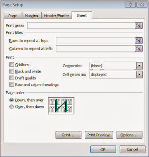
On the Page Layout ribbon, click on the Print Titles icon.

(In earlier versions of Excel, you can get to the same screen by choosing File, Page Setup and selecting the Sheet tab).

You will see the following window:

In the Print titles section, you can specify the rows you want to repeat at the top of every page by clicking in the “Rows to repeat at top:” box and selecting the rows that include your titles.

As you can see there is also a box to allow you to repeat columns if your print will straddle multiple pages horizontally. This is much less common, but can sometimes be useful.

Note that neither setting changes the spreadsheet that you see on the screen – just what is printed.

If you enjoyed this post, go to the top of the blog, where you can subscribe for regular updates and get two freebies “The 5 Excel features that you NEED to know” and “30 Chants for Better Charts”.

From the Not Just Numbers blog:

Obviously we all know how useful Excel is as a tool for work, but every now and again I come across a spectacular and unusual use of Excel, that I want to share with you.

Back in June, I posted some examples of the Excel art of Tatsuo Horiuchi.

This week I came across another amazing Excel artist by the name of Shukei. You can see some of Shukei’s work on the YouTube channel Shukeiart.

In the video below, you can see the whole process of creating an Excel painting of Yoda from Star Wars condensed into under three minutes!

Now that makes using Excel to create next year’s budget look pretty tame!

May the force be with you!

If you enjoyed this post, go to the top of the blog, where you can subscribe for regular updates and get two freebies “The 5 Excel features that you NEED to know” and “30 Chants for Better Charts”.

From the Not Just Numbers blog:

Sometimes we build an Excel spreadsheet that has a number of worksheets (or tabs) that are the same layout.

No matter how well we have designed our spreadsheet, there are times when we need to make updates. This can be further improvements or changes to reflect changing requirements.

This can be a time-taking task if the changes are to be made to multiple worksheets. Fortunately, Excel has a way to do this.

First of all, I think it is worth mentioning that some of the reasons we have multiple worksheets are due to bad spreadsheet design. For example, having a sheet for each month is not usually the best way to handle most applications. In most situations it is far better to have a sheet that contains all of the data and a report sheet that allows you to report that data for any month. For my advice on laying out data, take a look at this earlier post.

Assuming that you have decided that you do need multiple sheets (or that you already have them and are not going to spend your time changing a spreadsheet that works!), then you can make Excel apply the changes to each of the sheets that you want it to.

First of all, click on the tab name of the first of the sheets that you want to edit (as you normally would to make that the active sheet). Then, hold down the Ctrl key while you select the other sheets you want to edit too.

You should now see that the backgrounds of the tab names of the selected sheets are all white.

While these multiple sheets are selected in this way, any change you make to one of the sheets will be applied to them all.

The really important thing to remember though, is what you need to do when you’ve made the changes:

Right-click on the tab name of one of the selected sheets and click “Ungroup Sheets”

If you don’t do this, then you can imagine the chaos you can cause when you type anything into one of the sheets and it changes them all!

This can be really useful, as long as you remember that last step!

If you enjoyed this post, go to the top of the blog, where you can subscribe for regular updates and get two freebies “The 5 Excel features that you NEED to know” and “30 Chants for Better Charts”.

From the Not Just Numbers blog:

You may remember that back in May, I told you about some work I was doing as part of the ICAEW IT Faculty’s Excel Community Advisory Committee. The other committee members and I have been working towards a set of Excel Principles to be published by the ICAEW (the Chartered Accountancy body for England and Wales),

In my post back in May, I posted my initial contribution. This was then merged with the contributions of the rest of the committee. Over the past few months these have been argued about, compromised, honed and, in no small part due to the diplomatic skills of Paul Booth of the IT Faculty, improved, to arrive at a set of Twenty Principles that the whole committee can get behind.

This process has now reached the stage where the principles can be released into the wild, to get the views of the wider Excel world.

I have reproduced the headline principles, as they currently stand, below, but I would strongly recommend that you visit the ICAEW’s IT Counts website, where you can download the full document, including explanations and examples illustrating each principle, as well as join in the debate.

THE TWENTY PRINCIPLES IN BRIEF

The spreadsheet’s business environment

1. Determine what role spreadsheets play in your business, and plan your spreadsheet standards and processes accordingly.

2. Adopt a standard for your organisation and stick to it.

3. Ensure that everyone involved in the creation or use of spreadsheets has an appropriate level of knowledge and competence.

4. Work collaboratively, share ownership, peer review.

Designing and building your spreadsheet

5. Before starting, satisfy yourself that a spreadsheet is the appropriate tool for the job.

6. Identify the audience. If a spreadsheet is intended to be understood and used by others, the design should facilitate this.

7. Include an ‘About’ or ‘Welcome’ sheet to document the spreadsheet.

8. Design for longevity.

9. Focus on the required outputs.

10. Separate and clearly identify inputs, workings and outputs.

11. Be consistent in structure.

12. Be consistent in the use of formulae.

13. Keep formulae short and simple.

14. Never embed in a formula anything that might change or need to be changed.

15. Perform a calculation once and then refer back to that calculation.

16. Avoid using advanced features where simpler features could achieve the same result.

Spreadsheet risks and controls

17. Have a system of backup and version control, which should be applied consistently within an organisation.

18. Rigorously test the workbook.

19. Build in checks, controls and alerts from the outset and during the course of spreadsheet design.

20. Protect parts of the workbook that are not supposed to be changed by users.

If you enjoyed this post, go to the top of the blog, where you can subscribe for regular updates and get two freebies “The 5 Excel features that you NEED to know” and “30 Chants for Better Charts”.

From the Not Just Numbers blog:

We often use Excel to analyse data from elsewhere. This might be from another Excel spreadsheet, or a text file exported from another software tool – maybe your accounts package.

We all know that Excel is brilliant at this, but the job can be made significantly more difficult when the data we want to analyse is not in the best format for us to work with.

Earlier this year, I wrote a post on tidying up text in Excel. This can help sort out the format of individual fields to get them the way you want them, but what if the layout of the data itself not what you require.

If you are not sure how you want your data laid out to make it easy to analyse, this post might help.

One frustrating layout issue is when you are presented with data that is in rows where columns would be more useful, or vice versa – fortunately Excel has a simple solution.

Say we have some data that we want to paste into our spreadsheet as follows:

This data would be easier to analyse if we had one column per field, i.e. two columns of data rather than two rows.

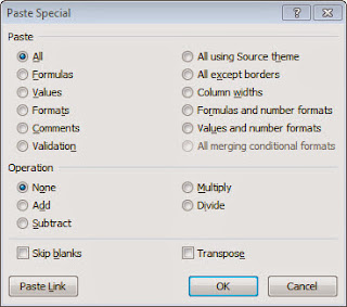
All we have to do is copy the data as normal but, when we paste it into our spreadsheet, click Paste Special, or Ctrl-Alt-V and we are presented with the following dialog box which allows us to make various changes to the data as we paste it (I will look at some of the others in future posts).

In this case we want to tick the Transpose box. This flips the data round, switching rows for columns.

When we then click OK, our pasted data looks like this:

Exactly as we wanted it.

If you enjoyed this post, go to the top of the blog, where you can subscribe for regular updates and get two freebies “The 5 Excel features that you NEED to know” and “30 Chants for Better Charts”.

From the Not Just Numbers blog:

Before we get into today’s tip, I’m aware that we have a lot of new visitors and subscribers and I thought it might be a good time to remind you of my needaspreadsheet.com service.

If you are reading this blog, then you probably use Excel in your job, and my posts are intended to help you to get the most out of this excellent tool. However, sometimes you might not have the time or the skills to get it to do what you want.

When that happens, you just need to enter what you need your spreadsheet to do in the form on the site, and I will send you a fixed price quote to build (or fix) your spreadsheet for you. The whole service is handled by email and as a result, your location really doesn’t matter – we have regular clients all over the globe.

Anyway, enough about me – on with today’s tip…

In an earlier post on tidying up text, I introduced the TRIM function, that removes all leading and trailing spaces from text, as well as ensuring that any spaces in the text are reduced to single spaces.

Whereas this is useful for many applications to tidy up data, sometimes we need to remove all spaces from text. This happened to me the other day with some client data from their bank account. The only way to ensure consistency of the data was to remove all spaces.

Thankfully, Excel has a function that can help with this, as well as a number of other issues we might face when manipulating text data.

The function we can use is SUBSTITUTE. This replaces all references to one string of text in a cell with another string of text.

Its syntax is:

=SUBSTITUTE(Text to apply the formula to,Old text,New text,[Instance number])

Text to apply the formula to – this can be text in inverted commas, but is usually a cell reference containing the text

Old text – the text that you wish to see replaced, this can be text (in inverted commas) or a reference to text

New text – the text that you wish to see Old text replaced with, this can be text (in inverted commas) or a reference to text

Instance number – this argument is optional (as indicated by the square brackets) and specifies which instance of Old text you wish to replace (1 for the first instance, 2 for the second, etc.). If this argument is not entered, the function replaces all instances of Old text.

We can use this function to remove all spaces from the text in cell A1, by entering the following in cell B1:

=SUBSTITUTE(A1,” “,””)

Note that the second argument is a space in inverted commas, whereas the third argument has no space.

B1 will now be the same as A1, but we will have replaced all instances of a space with nothing – i.e. removing all of the spaces.

It’s as simple as that.

If you enjoyed this post, go to the top of the blog, where you can subscribe for regular updates and get two freebies “The 5 Excel features that you NEED to know” and “30 Chants for Better Charts”.

From the Not Just Numbers blog:

Before we crack on with this week’s post, just a quick little note about Mynda Treacy’s Excel Dashboards course.

I know that many of you have purchased the course and taken advantage of the early bird discount. As when we offered the course last time, the course has been very popular and the feedback has been excellent.

If you haven’t already done so, you can still get the course until 30th October and, although you have missed the discount, the course still represents excellent value and I will still throw in my Introduction to Pivot Tables course free of charge.

You can get the course here.

OK, on with this week’s tip. We all know how to sum a list of numbers, but Excel offers a number of other functions for analysing a list, and today I want to introduce two of them that enable you to find the maximum or minimum value in a list.

This could be useful for all sorts of reasons – finding the maximum sales in any particular month, or the lowest score achieved in a test, for example.

Excel offers a simple way of doing this with the MAX and MIN functions.

Both functions have the following syntax:

=MAX(number1,number2,etc.) you can have as many numbers as you like in this list.

So, for example:

=MAX(23,45,12,65,21)  will return 65

and

=MIN(23,45,12,65,21)  will return 12

These numbers can be cell references, or ranges of cells – and this is usually of far more practical use.

So, say the cells A1 to A5 contain the numbers 23,45,12,65 and 21, then:

=MAX(A1:A5)  will return 65

and

=MIN(A1:A5)   will return 12

And that’s really all you need to know.

If you enjoyed this post, go to the top of the blog, where you can subscribe for regular updates and get two freebies “The 5 Excel features that you NEED to know” and “30 Chants for Better Charts”.

From the Not Just Numbers blog:

Before we get into today’s post, just a little reminder that the 20% discount offer on Mynda Treacy’s Excel Dashboards course expires on Thursday. So if you’ve been thinking about it, now’s the time to do something about it, if you want to save some money.

Today’s post is a follow-up to an earlier post, “Do you really need to merge those cells?” where I highlighted the dangers of merging cells.

It became clear in some of the comments on forums that I had highlighted the problems but had been less than clear on alternatives.

This post is intended to address that.

Just to recap, the problems highlighted in that earlier post were:

• Data containing merged cells can not be treated like a normal data table – meaning that we can’t use all of the tools that we might want to use for referring to a properly formatted data table, such as pivot tables, SUMIF, etc;
• Copying and pasting ranges is restricted to those with cells merged in the same way;
• Fill down doesn’t work if any of the cells in the range to be filled are merged;
• Even if we unmerge all of the cells, this rarely solves the problem, as this action will assume that the merged cell contents should be placed in the top left cell of the unmerged range – which may not be where you want them to be. Also, having done this, it is often not clear where your data is, as the labels may now be in a completely different place.

If you enjoyed this post, go to the top of the blog, where you can subscribe for regular updates and get two freebies “The 5 Excel features that you NEED to know” and “30 Chants for Better Charts”.

From the Not Just Numbers blog:

Mynda Treacy’s excellent Excel Dashboards online course is once again open for registration and once again there is an excellent offer for those of you who don’t hang about – more about that later in this post.

Back in July, Mynda wrote a guest post for me on the subject of Excel Dashboards, which you can read here. This is becoming a very important skill and is often now required by employers. Mynda’s post is a really good introduction and if, for whatever reason, you do not take up the offer on the training course, I would recommend that you at least read Mynda’s guest post.

Charts

To celebrate the re-opening of Mynda’s course, I have arranged to offer her eBook, 30 Chants for Better Charts, absolutely free to subscribers.

Many of us use charts regularly in our work, but few of us do it well, and Mynda’s eBook provides some excellent tips on how best to format charts so that they look professional and convey the information that they are supposed to, clearly.

If you’re not already a subscriber to Not Just Numbers, simply enter your name and email address in the box at the top right of the blog and you will receive Mynda’s eBook, as well as other freebies, and updates on new posts to the blog.

Excel Dashboards

The Excel Dashboards course is video based and available online 24/7. It comes with comprehensive Excel workbooks and several sample dashboards to keep. There’s also an option to download the videos, plus Mynda personally provides support for the first 6 weeks of the 12 month membership.

Disclosure: I make a small commission for students who join Mynda’s course, but as you know I don’t just recommend anything and everything. It has to be of outstanding quality and value, and something I can genuinely recommend. After all, if doesn’t live up to what I’ve promised you’ll think poorly of me too and I don’t want that. Oh, and just watching the course videos won’t transform your career, you have to actually put it into practice, but then you know that.

If you enjoyed this post, go to the top of the blog, where you can subscribe for regular updates and get your free report “The 5 Excel features that you NEED to know”.