 From the Not Just Numbers blog:
This week, I want to show you a neat little trick for doing something a little more visually interesting than just using brackets to distinguish between positive and negative variances.
In this post, I will show you how to automatically show a green thumbs up or a red thumbs down next to the variance (depending on whether it is good or bad).
Once you know how to do this you can replace these with arrows or some other symbols and make the colours whatever you want them to be.
OK. Say we have an actual figure in cell A1 and a comparison in cell B1. A1 might be this month’s sales, for example, and B1 might be budgeted sales, or last month’s sales. Either way, we want to make it obvious at a glance that A1 being higher than B1 is a good thing, and A1 being less than B1 is a bad thing.
A green thumbs up, or a red thumbs down, in cell C1, should make this pretty clear – so how do we do it?
First of all, where do we get the Thumbs Up and Thumbs Down symbols from?
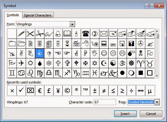
We can discover what symbols are available in different fonts by selecting Symbol from the Insert ribbon (this is on the far right of the standard Insert ribbon).
If we select the Wingdings font from the drop-down at the top, you can see there is a Thumbs Up symbol there. Click on it and note the number at the bottom left after the name of the font. In this case it says “Wingdings: 67”, so the number to note is 67. This is the character code of this symbol. Click on the Thumbs Down and you will see that this has a character code of 68.
OK, now cancel this screen, as we are going to insert these symbols in a different way – now we know what we want.
We can refer to any character by its character code using the CHAR function. So, if in any particular cell, we change the font to Wingdings (either by right-clicking and using the format cells dialog box, or by selecting the Wingdings font from the drop-down on the Home ribbon),
=CHAR(67)
will return the Thumbs Up symbol.
For our purposes, set the font in cell C1 to Wingdings and type the following formula into cell C1,
=IF(A1>=B1,CHAR(67),CHAR(68))
This formula will return the Thumbs Up character if A1 is greater than or equal to B1, and the Thumbs Down character, if it is not.
If you need a refresher on the IF function, take a look at this earlier post.
All we need to do now is change its colour. We can do this using Conditional Formatting.
First of all, change the font colour in cell C1 to green (again, either from th Home ribbon or Format Cells).
We then want this to change to red if C1 contains a Thumbs Down.
Click on cell C1 and from the Home ribbon, click Conditional Formatting, New Rule, Use a formula to determine which cells to format (this step is covered in more detail in this earlier post).
In the formula box, enter:
=C1=CHAR(68)
and click on the Format button to change the font colour to red.
That’s it. Change the values in A1 an B1 and you will see C1 change from a green Thumbs Up to a red Thumbs Down, depending on whether A1 is greater or less than B1!
As I said earlier in the post, you could use other symbols, such as up and down arrows and other colours, depending on your requirements. Have fun with it!
If you enjoyed this post, go to the top of the blog, where you can subscribe for regular updates and get two freebies “The 5 Excel features that you NEED to know” and “30 Chants for Better Charts”.


