From the Not Just Numbers blog:
I recently created a spreadsheet for tracking gambling debts for a client who wanted to enter (and display) odds as a fraction.
This required me to come up with a formula to read the fraction so that it could be used in the calculation of the winnings.
This got me to thinking that there will be other scenarios where it is preferable to enter numbers as fractions rather than decimals – and to display them as such.
So I thought I’d share my approach.
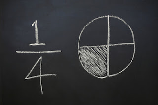
The easy bit is to get it to allow the user to type in a fraction and continue to display it as such. Simply change the number format of the input cells to Text, so that when the user types 1/4, that is what is displayed. A general format should also do this but it is better to format exactly what you are after rather than use General and let Excel decide.
The tricky bit is to get Excel to convert this to something it can use in calculations – i.e. a decimal.
The method I used was to use text manipulation formula to split out the components of the fraction.
The functions needed are VALUE, LEFT, RIGHT, LEN and FIND.
RIGHT, LEFT and LEN are all described in an earlier post:
Excel Tip: Manipulating text in Microsoft Excel
so I won’t described them again here.
The two functions not covered in that post are:
VALUE(text) converts a number formatted as text into a number that Excel can then use in calculations. My first attempt was to use this to convert the fraction straight to a decimal number, however it requires the text to be a single number – not a formula. It can, however, be used to convert the numerator and the denominator into numbers.
FIND(text to find,text to search in,optional starting position) returns the position (as a number) of the first instance of the string text to find, in the string text to search in starting at theoptional starting position if specified. e.g. FIND(“D”,”ABCDEFEDCBA”,5) returns 8 as this is the position of the first D it finds from position 5 onward – whereas FIND(“D”,”ABCDEFEDCBA”) returns 4 as it starts looking at the start of the string.
We basically want to return the value of the text before the slash and divide it by the text after the slash, to give us a number we can use. We will assume the fraction is entered in cell A1.
In both cases we will need to find the position of the slash, using =FIND(“/”,A1).
We can return the text before the slash by using the LEFT function:
=LEFT(A1,FIND(“/”,A1)-1) (without the -1 we would return the slash as well, which we don’t want)
We can then convert this to a value using the VALUE function:
=VALUE(LEFT(A1,FIND(“/”,A1)-1))
We can return the text after the slash by using the RIGHT function, but we will need to use LEN to know where to stop:
The number of characters we will need to return in the RIGHT function, can be calculated as follows:
=LEN(A1)-FIND(“/”,A1)
So the RIGHT function then reads:
=RIGHT(A1,LEN(A1)-FIND(“/”,A1))
We can again use the VALUE function to convert this to a number:
=VALUE(RIGHT(A1,LEN(A1)-FIND(“/”,A1)))
Finally, divide one by the other to convert the whole fraction to a usable number:
=VALUE(LEFT(A1,FIND(“/”,A1)-1))/VALUE(RIGHT(A1,LEN(A1)-FIND(“/”,A1)))
Definitely a good idea to put this into a working cell, so that you don’t need to do this every time you want to use the fraction. All of your formulae can then refer to the calculated cell.
I’m sure some of you will have other approaches which I’d love to hear about in the comments.
Click here for our our exclusive offer on Online Excel Training
If you enjoyed this post, go to the top of the blog, where you can subscribe for regular updates and get your free report “The 5 Excel features that you NEED to know”.

