From the Not Just Numbers blog:
One of my ten principles last week was to protect cells with formulae in them, and it occurred to me that it might be useful to do a quick post on how cell protection works.
It is really easy to use and very effective for ensuring that formulae don’t get over-typed.
Protecting cells is a two-stage process:
First of all we choose which cells we want to be locked, and then we switch protection on for that worksheet.
Setting which cells are to be protected
We determine the protection status of a cell by selecting a cell, or cells, and choosing “Format Cells”. This can be accessed from the right-click menu.
The final tab of the window is Protection:
By default, all cells have the Locked box ticked (as shown above). This means that the cell will be locked (and therefore can’t be edited) if the sheet is protected (in the next stage).
If we untick this box, then the cell, or cells, will remain free to edit, when protection is switched on.
We will typically select the data entry cells and unlock them in this way, prior to switching protection on for the sheet.
There is also a second tick box (Hidden) that allows you to hide the formula in the cell (again, only once protection is switched on).
Switch Protection on for the worksheet
In Excel 2007 onwards select the Review ribbon and click Protect Sheet. In earlier versions of Excel, select Tools->Protection->Protect Sheet.
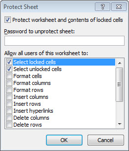
In both cases you will see the following:
The top tick box will always be ticked (you can’t click OK if it isn’t).
Under that, you can choose to enter a password that will be required to unprotect the sheet. You will be asked to enter this twice to avoid mistyping it.
Below that is a list of tick boxes where you can allow things that would otherwise not be allowed on a protected sheet. By default, the first two are ticked, meaning that you are still allowed to select any cells (whether locked or unlocked). On a data entry screen, I often untick the top box, as this stops the user even clicking in cells that can’t be edited – making it easier to navigate the sheet.
Other tickboxes (further down the list) that you may want to tick, are such things as allowing the use of Autofilter, Sort, or Pivot Tables. This form gives quite a lot of control over what the user can or can’t do.
When you are happy with the above, click OK. The protection settings will be applied to the active Worksheet.
To unprotect the sheet again, go to the same place as you did to protect it. You will notice that the option now says Unprotect Sheet. When you click this, you will be asked for the password (if you applied one), and then the sheet will be unprotected again.
If you then go to protect it again, the tick box options are remembered, however you will need to set the password again.
And that’s cell protection!
Click here for our our exclusive offer on Online Excel Training
If you enjoyed this post, go to the top of the blog, where you can subscribe for regular updates and get your free report “The 5 Excel features that you NEED to know”.


