 From the Not Just Numbers blog:
It’s been a while since I covered GETPIVOTDATA on the blog, so I thought it was worth a re-visit, but with the specific objective of demonstrating a structured approach to populating a fixed layout report, with data pulled from a pivot table.
NB: This post assumes that you already have, or know how to create, a pivot table containing your data. If not, you might find my video training course on the subject useful.
A very common example of this type of application is monthly management accounts: A pivot table can be great for doing the analysis and producing the numbers for the accounts, but these usually then need to be presented in a particular monthly accounts pack template.
This post will explain how to populate any fixed report with data pulled from a pivot table. This can be a great way of automatically populating any existing report that you might currently be populating manually.
One question that I am sure some readers will ask is “Why not use SUMIF and skip the pivot table altogether?”
This is a fair question and I sometimes take that approach, however one big advantage of the pivot table step is that you get to see ALL of the data summarised and can identify any data that is not appearing on the final report – SUMIFs on the other hand will only show what you look for, but you will not see any new categorisations that are not on the final layout (for example, a new nominal ledger code). Also, it is much easier to trace how a number is made up using the pivot table approach.
Let us take the pivot table report we produced in my cash book post:
NB: I have made one slight tweak to the one produced in that post, in that I have moved the year and month to be columns rather than report filter fields. This means that all years and months will appear as data is added, and our final report can pull out the month required.
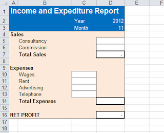
The final template we use looks like this, and we normally key in the numbers from the pivot table (in reality, this might be a 30-page management accounts pack, but the principles are just the same as in our simple example):
Our objective is to automatically populate this in a structured way, from the pivot table.
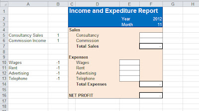
We need to do a little preparation on the final report, by inserting 2 columns to the left of the report (these can be hidden, or kept outside of the print area, once we are finished).
In the first column, on the rows we need to populate, we enter exactly how that row is described in the pivot table. In the second column, we enter a 1 or a -1, depending whether we want to reverse the sign on that row or not.
So the report sheet now looks like this:
We will now build a formula that can be copied into every cell that we want to pull data into. We will create the formula in cell F5 and copy it to the others (NB: The totals are all just simple sums and are already in the template).
If you remember from my earlier posts on GETPIVOTDATA, the syntax of the function is as follows:
=GETPIVOTDATA(“Name of data field to return”,location of pivot table,”field1″,”item1″,”field2″,”item2″)
Where:
Name of data field to return is a text field, being the name of the pivot table field as it appears on the pivot table.
location of pivot table is a reference to a cell anywhere within the pivot table, it is often best to use the top left cell of the main body of the pivot table, as this will remain in a constant position no matter how much the data changes.
field1, item1,field2,item2,etc. are pairs of field and item names from the row, column or page (filter) areas of the pivot table. You can use as many pairs as you like. The field name comes from the original column heading in the data, the item name is the entry in that column that creates a unique row, column or page in the pivot table.
SO to return the figure we want, being the commission sales figure for month 11 of the year 2012, the GETPIVOTDATA formula would be:
=GETPIVOTDATA(“Value”,’Income and Expenditure’!$A$4,”Expense/Income Name”,”Consultancy Sales”,”Year”,2012,”Month”,11)
i.e. return the total of the field Value, from the Pivot Table at ‘Income and Expenditure’!$A$4 where Expense/Income Name is “Consultancy”, Year is 2012 and Month is 11.
For this formula to be able to be used throughout we need to change the values to references.
We can swap “Consultancy Sales” for $A5 (notice we place a dollar sign before the A, so that if we copy the formula to a different column, it will still look in column A for the Expense/Income Name).
We can swap 2012 for $F$2 (here we have used the dollar signs to fix both the row and the column as the year will always be in cell F2).
Finally we can swap 11 for $F$3.
So our new formula is:
=GETPIVOTDATA(“Value”,’Income and Expenditure’!$A$4,”Expense/Income Name”,$A5,”Year”,$F$2,”Month”,$F$3)
There are a couple of additional changes that we need to make to complete the formula before we copy it to the other cells.
This formula works great if there is a figure in the pivot table for the year, month and category in question, but will return an error otherwise, so we need to catch that and return a zero. I covered this in a post a couple of years ago (EXCEL TIP: Eliminating #DIV/0! and other errors automatically using ISERROR). In later versions of Excel, you can use IFERROR to replace the two functions IF and ISERROR, however I don’t see that this makes the formula any simpler, yet stops it working in earlier versions, so we will stick to IF and ISERROR here. The new formula is now:
=IF(ISERROR(GETPIVOTDATA(“Value”,’Income and Expenditure’!$A$4,”Expense/Income Name”,$A5,”Year”,$F$2,”Month”,$F$3)),0,GETPIVOTDATA(“Value”,’Income and Expenditure’!$A$4,”Expense/Income Name”,$A5,”Year”,$F$2,”Month”,$F$3))
Finally, we need to reflect the column we added to allow us to reverse the sign. In our example, the pivot table has sales (credits) as a positive and expenses (debits) as a negative (if this had come from a traditional trial balance, they would have been the other way around). In our final report, we want to show both as positives and the totals will deduct expenses from sales, so we have entered 1 against the rows that we want to keep with the same sign and -1 against the expenses, where we want to reverse the sign.
This is simple to reflect in the formula as we just need to multiply the result by column B:
=IF(ISERROR(GETPIVOTDATA(“Value”,’Income and Expenditure’!$A$4,”Expense/Income Name”,$A5,”Year”,$F$2,”Month”,$F$3)),0,GETPIVOTDATA(“Value”,’Income and Expenditure’!$A$4,”Expense/Income Name”,$A5,”Year”,$F$2,”Month”,$F$3))*$B5
Note that we have again used the dollar sign to fix the column, but not the row.
We can now copy this formula into cells F6 and E10 to E13.
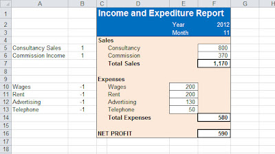
Our final report now looks like this:
The numbers will now all automatically update if the pivot table changes or if the year and/or month are changed at the top.
This approach works with far more complex reports than this and can be expanded to allow for multiple value fields in the pivot and multiple columns in the final report.
I use this approach regularly to automatically populate existing reports for clients. They often have very elaborate reports that take ages to complete manually. With this approach, I can insert a couple of columns and work out the formula, without changing the look of their report at all.
Go on, revisit all of those manual reports now. You’ll be glad you did when next month end comes around!
If you enjoyed this post, go to the top of the blog, where you can subscribe for regular updates and get your free report “The 5 Excel features that you NEED to know”.


