 From the Not Just Numbers blog:
I have previously blogged about how to create a drop-down list in Excel using data validation, but sometimes I am asked to make the options in one drop-down list dependent on the selection from another.
This can be done pretty simply if all you want to do is present different lists based upon the selection from the first drop-down.
For example, we might have a drop-down to choose product group and then a second drop-down to choose an actual product from that group. In the second drop-down, we want to only show the products in the chosen product group.
So here goes…
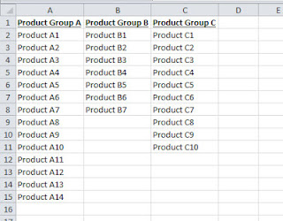
The first task is to layout the lists in a way that makes this possible:
As you can see above , we have entered the product groups along row 1, with the products contained in each below them.
We then need to name the following ranges on this sheet as follows:
GroupList A1:C1
ProductList1 A2:A51
ProductList2 B2:B51
ProductList3 C2:C51
I have assumed that we only have 3 product groups and up to 50 products in each, but obviously these can be changed to suit the data.
We then want to create the two drop-downs on a separate sheet – let’s say in cells A1 and B1.
The Product Group drop-down in cell A1 is just an ordinary drop-down, where we select Data Validation -> List and enter =GroupList in the Source box (my earlier post explains this in more detail).
The second drop-down is the one that does the work. I will tell you what we do first and then explain it.
In cell B1 (where we want the product drop-down), we again select Data Validation -> List but this time enter the following into the Source box:
=INDIRECT(“ProductList”&MATCH(A1,GroupList,0))
we should also untick Ignore blank as there are blank cells in the product ranges we selected. If we leave this ticked, Excel will still present the drop-down list, but allow anything to be typed into the cell.
That’s the job done – this will now provide a drop-down of the right products for the chosen product group.
So, what is this formula doing?
There are three elements that we need to understand to decipher the formula:
=INDIRECT() forces Excel to recognise whatever is contained in the brackets as an address or range. We have applied this to the formula so that the Data Validation source box recognises that this is a range, rather than a piece of text.
=MATCH(A1,GroupList,0) searches for the value A1, within the range GroupList. The third argument (0) tells the function that it should only look for an exact match. The result is the position as a number, i.e. if it finds A1 in the first cell of GroupList, it returns 1, etc.
The & symbol combines two pieces of text together into one string.
Putting all three together, if cell A1 was to contain “Product Group B”, then the Match formula would return 2 (as this appears in the second cell of GroupList).
So “ProductList”&MATCH(A1,GroupList,0) = the text string “ProductList2”
and =INDIRECT(“ProductList2”) is therefore the range named ProductList2, i.e. the range name we gave to the list of products in Product Group B.
Obviously, the names of the ranges can be changed depending on the data, as long as the dependent list ranges all end with their position.
If you enjoyed this post, go to the top of the blog, where you can subscribe for regular updates and get your free report “The 5 Excel features that you NEED to know”.

