From the Not Just Numbers blog:
Just a short post today on a very useful use for the VLOOKUP function.
Typically when we use VLOOKUP, we are looking for an exact match from a list. For example, we might look up a customer’s address, based upon their account code.
But what if we want to look up the correct commission rate or tax rate, based upon what earnings band a particular value falls into?
VLOOKUP handles this extremely well, when you understand its mysterious fourth (optional) argument.
The syntax of a VLOOKUP function is:
First of all though, let us outline the problem with an example.
We have a cell (D2) containing an income figure upon which we need to calculate a sales commission.
However, the rate of commission changes depending on the size of the income figure as follows:
0 – 9,999 pays 10%
10,000 – 49,999 pays 20%
and 50,000+ pays 25%
How do we calculate what rate to use?
We could use IF statements, however this falls down with more bands and is very inflexible when it comes to changing the bands. A far better solution is to use the VLOOKUP function.
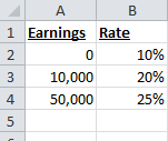
We need to create a two column table with the start of the band in the first column, and the rate to use in the second. This table must be in ascending order of earnings, i.e.
When we set the final argument in the VLOOKUP to TRUE (or leave it blank), it scans the lookup table for the highest earnings value that is still less than the lookup value, so:
=VLOOKUP(D2,A2:B4,2,TRUE)
will return the rate we are looking for.
We can also use exactly the same approach for other similar problems, such as looking up tax rates.
If you enjoyed this post, go to the top of the blog, where you can subscribe for regular updates and get your free report “The 5 Excel features that you NEED to know”.


